Quantum computing explained with cats
$$\newcommand{\ket}[1]{\mid#1 \rangle}$$
Bits as cats
A bit can be either 0 or 1. Let us represent them by cats:
bit = 0  bit = 1
Qubits
Qubits are quantum bits. They are also represented by cats, but they can be in a superposed state. For instance:
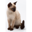
is the qubit equal to 0. This state is denoted by |0>.
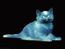
is the qubit equal to |1>.
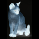
represents the superposition $$\frac 1
{\sqrt 2} (\ket 0 +
\ket 1)$$ where the qubit is at |0> with probability 1/2 and at |1> with probability 1/2.
represents the superposition $$\frac
1 2 \ket 0 + \frac
{\sqrt 3} 2 \ket 1)$$ where the qubit is at |0> with probability 1/4 and at |1> with probability 3/4.
Two qubits
 represents the superposition $$\frac 1 2 (\ket {00} + \ket {01} + \ket {10} + \ket
{11})$$ where all states |00>, |01>, |10> and |11> have probability 1/4.
is a Bell state: it may be the
superposition $$\frac 1 {\sqrt 2} (\ket {00} + \ket {11})$$ where we have |00> with probability 1/2 and |11>
with
probability 1/2. There is entanglement.
represents the superposition $$\frac 1 2 (\ket {00} + \ket {01} + \ket {10} + \ket
{11})$$ where all states |00>, |01>, |10> and |11> have probability 1/4.
is a Bell state: it may be the
superposition $$\frac 1 {\sqrt 2} (\ket {00} + \ket {11})$$ where we have |00> with probability 1/2 and |11>
with
probability 1/2. There is entanglement.
Note: in fact scalars (i.e. numbers) are complex numbers
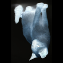
For instance, if the scalar is negative,
images are turned.
 represents the superposition -|1>.
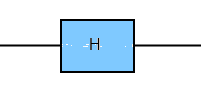
Hadamard gates
Hadamard gates enables to compute uniform
superpositions of all physical states.
The problem of finding a specific solution
Let f be a
function from \(\{0, 1\}^n\) to {0, 1}. Here n = 4. We pose \(N = 2^n\). Here N =
16. There is a unique element x such that f(x) = 1.
In the rest of this paper, consider x = 0101 to be that unique element, i.e.

 .
The aim is to find x without any knowledge on f. More precisely, the problem that we will solve is defined
as follows:
.
The aim is to find x without any knowledge on f. More precisely, the problem that we will solve is defined
as follows:
- input: a black box Uf that computes f;
- output: x such that f(x) = 1.
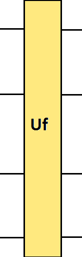
A gate for Uf
The black box is constructed so that it preserves all physical states except |0101>, which is mapped to -|0101>.
We suppose that \(U_f(x) = -x\) when f(x) = 1 and Uf(x) = x for all other x.
For all other elements, the gate outputs its input.
Grover's algorithm
Grover's algorithm solves the problem of finding a specific solution (see also this link).
The circuit of that algorithm is as follows.
Grover's starts with 0000.
Then we apply Hadamar gates to obtain a uniform superposition of all physical states.
We then repete a sequence of Uf and D (explained below).
After an appropriate number of repetitions (not too many, not little), the probability to read our unique element is very high, see (*).
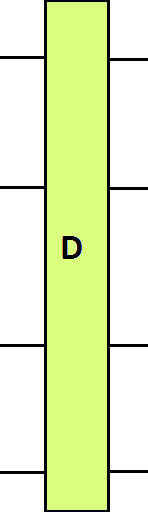
It remains to describe D and to see what is the optimal number of repetition of Uf D. Actually, D is the Grover diffusion
operator that amplifies the unique state that has a negative scalar and put a positive scalar on it that is stricly
greater in norm that the previous scalar. The other states are such that their probability are lower. In other
words, the state |0101> is amplified.
When we then apply again the Uf operator, we continue to negate the scalar of |0101> and the other scalars are kept
equal. Then D continues to amply more and more the scalar of |0101> in norm.
After some iterations of Uf
and D, we may measure the qubits and obtain |0101> with a probability
higher than 1/2: at (*) in the circuit the measure is ideal.